CNN In Pytorch

Pytorch에는 CNN을 개발 하기 위한 API들이 있습니다. 다채널로 구현 되어 있는 CNN 신경망을 위한 Layers, Max pooling, Avg pooling 등, 이번 시간에는 여러 가지 CNN을 위한 API를 알아 보겠습니다. 또한, MNIST 데이터 또한 학습 해 보겠습니다.

MNIST Example

Convolution Layers

Convolution 연산을 위한 레이어들은 다음과 같습니다.

Conv1d (Text-CNN에서 많이 사용)
Conv2d (이미지 분류에서 많이 사용)
Conv3d

위 3가지 API들은 내부 원리는 다 같습니다. 이번에는 자주 사용하는 Conv2d를 중점으로 설명 하도록 하겠습니다.

Parameters

일단 Conv2d(in_channels, out_channels, kernel_size, stride=1, padding=0, dilation=1, groups=1, bias=True, padding_mode='zeros')의 파라미터는 다음과 같습니다.

in_channels: 입력 채널 수을 뜻합니다. 흑백 이미지일 경우 1, RGB 값을 가진 이미지일 경우 3 을 가진 경우가 많습니다.
out_channels: 출력 채널 수을 뜻합니다.
kernel_size: 커널 사이즈를 뜻합니다. int 혹은 tuple이 올 수 있습니다.
stride: stride 사이즈를 뜻합니다. int 혹은 tuple이 올 수 있습니다. 기본 값은 1입니다.
padding: padding 사이즈를 뜻합니다. int 혹은 tuple이 올 수 있습니다. 기본 값은 0입니다.
padding_mode: padding mode를 설정할 수 있습니다. 기본 값은 'zeros' 입니다. 아직 zero padding만 지원 합니다.
dilation: 커널 사이 간격 사이즈를 조절 합니다. 해당 링크를 확인 하세요.
groups: 입력 층의 그룹 수을 설정하여 입력의 채널 수를 그룹 수에 맞게 분류 합니다. 그 다음, 출력의 채널 수를 그룹 수에 맞게 분리하여, 입력 그룹과 출력 그룹의 짝을 지은 다음 해당 그룹 안에서만 연산이 이루어지게 합니다.
bias: bias 값을 설정 할 지, 말지를 결정합니다. 기본 값은 True 입니다.

Shape

Input Tensor $(N, C_{in}, H_{in}, W_{in})$ 의 모양과 Output Tensor $(N, C_{out}, H_{out}, W_{out})$ 의 모양은 다음과 같습니다.

Input Tensor $(N, C_{in}, H_{in}, W_{in})$

$N$ : batch의 크기
$C_{in}$ : in_channels에 넣은 값과 일치하여야 함.
$H_{in}$ : 2D Input Tensor의 높이
$W_{in}$ : 2D Input Tensor의 너비

Output Tensor $(N, C_{out}, H_{out}, W_{out})$

$N$ : batch의 크기
$C_{out}$ : out_channels에 넣은 값과 일치 함.
$H_{out} = \lfloor{H_{in} + 2 \times padding[0] - dilation[0] \times (kernel\_size[0] - 1) - 1 \over stride[0]} + 1\rfloor$
$W_{out} = \lfloor{W_{in} + 2 \times padding[1] - dilation[1] \times (kernel\_size[1] - 1) - 1 \over stride[1]} + 1 \rfloor$

Code Example

import torch
import torch.nn as nn
import torch.nn.functional as F

class CNN(nn.Module):
  def __init__(self):
    super(CNN, self).__init__()
    self.conv1 = nn.Conv2d(in_channels=1, out_channels=3, kernel_size=5, stride=1)
    self.conv2 = nn.Conv2d(in_channels=3, out_channels=10, kernel_size=5, stride=1)
    self.fc1 = nn.Linear(10 * 12 * 12, 50)
    self.fc2 = nn.Linear(50, 10)
  
  def forward(self, x):
    print("연산 전", x.size())
    x = F.relu(self.conv1(x))
    print("conv1 연산 후", x.size())
    x = F.relu(self.conv2(x))
    print("conv2 연산 후",x.size())
    x = x.view(-1, 10 * 12 * 12)
    print("차원 감소 후", x.size())
    x = F.relu(self.fc1(x))
    print("fc1 연산 후", x.size())
    x = self.fc2(x)
    print("fc2 연산 후", x.size())
    return x

cnn = CNN()
output = cnn(torch.randn(10, 1, 20, 20))  # Input Size: (10, 1, 20, 20)

Out

연산 전 torch.Size([10, 1, 20, 20])
conv1 연산 후 torch.Size([10, 3, 16, 16])
conv2 연산 후 torch.Size([10, 10, 12, 12])
차원 감소 후 torch.Size([10, 1440])
fc1 연산 후 torch.Size([10, 50])
fc2 연산 후 torch.Size([10, 10])

Pooling Layers

Pooling 연산을 위한 레이어 들은 다음과 같습니다.

MaxPool1d
MaxPool2d
MaxPool3d
AvgPool1d
AvgPool2d
AvgPool3d

위 6가지 API들은 차원 수, Pooling 연산의 방법을 제외하곤 다 같습니다. 대표적인 MaxPool2d를 설명 해 보겠습니다.

Parameters

일단 MaxPool2d(kernel_size, stride=None, padding=0, dilation=1, return_indices=False, ceil_mode=False)의 파라미터는 다음과 같습니다.

kernel_size: 커널 사이즈를 뜻합니다. int 혹은 tuple이 올 수 있습니다.
stride: stride 사이즈를 뜻합니다. int 혹은 tuple이 올 수 있습니다. 기본 값은 1입니다.
padding: zero padding을 실시 할 사이즈를 뜻합니다. int 혹은 tuple이 올 수 있습니다. 기본 값은 0입니다.
dilation: 커널 사이 간격 사이즈를 조절 합니다. 해당 링크를 확인 하세요.
return_indices: True 일 경우 최대 인덱스 를 반환합니다.
ceil_mode: True 일 경우, Output Size에 대하여 바닥 함수대신, 천장 함수를 사용합니다.

Shape

Input Tensor $(N, C_{in}, H_{in}, W_{in})$ 의 모양과 Output Tensor $(N, C_{out}, H_{out}, W_{out})$ 의 모양은 다음과 같습니다.

Input Tensor $(N, C, H_{in}, W_{in})$

$N$ : batch의 크기
$C$ : channel의 크기.
$H_{in}$ : 2D Input Tensor의 높이
$W_{in}$ : 2D Input Tensor의 너비

Output Tensor $(N, C, H_{out}, W_{out})$

$N$ : batch의 크기
$C$ : channel의 크기.
$H_{out} = \lfloor{H_{in} + 2 \times padding[0] - dilation[0] \times (kernel\_size[0] - 1) - 1 \over stride[0]} + 1\rfloor$
$W_{out} = \lfloor{W_{in} + 2 \times padding[1] - dilation[1] \times (kernel\_size[1] - 1) - 1 \over stride[1]} + 1 \rfloor$

Code Example

import torch
import torch.nn as nn
import torch.nn.functional as F

class CNN(nn.Module):
  def __init__(self):
    super(CNN, self).__init__()
    self.max_pool1 = nn.MaxPool2d(kernel_size=2)
    self.max_pool2 = nn.MaxPool2d(kernel_size=2)
    self.fc1 = nn.Linear(10 * 5 * 5, 50)
    self.fc2 = nn.Linear(50, 10)
  
  def forward(self, x):
    print("연산 전", x.size())
    x = F.relu(self.max_pool1(x))
    print("max_pool1 연산 후", x.size())
    x = F.relu(self.max_pool2(x))
    print("max_pool2 연산 후",x.size())
    x = x.view(-1, 10 * 5 * 5)
    print("차원 감소 후", x.size())
    x = F.relu(self.fc1(x))
    print("fc1 연산 후", x.size())
    x = self.fc2(x)
    print("fc2 연산 후", x.size())
    return x

cnn = CNN()
output = cnn(torch.randn(10, 1, 20, 20))

Out

연산 전 torch.Size([10, 1, 20, 20])
max_pool1 연산 후 torch.Size([10, 1, 10, 10])
max_pool2 연산 후 torch.Size([10, 1, 5, 5])
차원 감소 후 torch.Size([1, 250])
fc1 연산 후 torch.Size([1, 50])
fc2 연산 후 torch.Size([1, 10])

MNIST 모델 학습

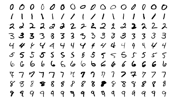
일단 MNIST 모델을 불러오기 위해서는 torchvision의 설치가 선행 되어야 합니다.

pip install torchvision

torchvision을 설치한 후, 필요한 라이브러리를 import 합니다.

import torch
import torch.nn as nn
import torch.nn.functional as F
import torch.optim as optim
from torchvision import datasets, transforms

MNIST 데이터를 가져오기 위해, datasets를 사용 하고, 이를 Tensor 객체로 가공 하기 위해, transforms를 사용합니다. Compose 함수를 이용해, Tensor로 가공 후, 정규화 또한 진행합니다. MNIST 데이터를 배치 학습 시키기 위해, DataLoader를 사용 합니다.

train_data = datasets.MNIST('./data/', train=True, download=True, transform=transforms.Compose([
        transforms.ToTensor(),
        transforms.Normalize((0.1307,), (0.3081,))
    ])) # 학습 데이터
train_loader = torch.utils.data.DataLoader(dataset=train_data, batch_size=50, shuffle=True)

test_data = datasets.MNIST('./data/', train=False, transform=transforms.Compose([
        transforms.ToTensor(),
        transforms.Normalize((0.1307,), (0.3081,))
    ])) # 테스트 데이터
test_loader = torch.utils.data.DataLoader(dataset=test_data, batch_size=50, shuffle=True)

CNN 클래스를 선언해 줍니다.

class CNN(nn.Module):
    def __init__(self):
        super(CNN, self).__init__()
        self.conv1 = nn.Conv2d(in_channels=1, out_channels=20, kernel_size=5, stride=1)
        self.conv2 = nn.Conv2d(in_channels=20, out_channels=50, kernel_size=5, stride=1)
        self.fc1 = nn.Linear(4 * 4 * 50, 500)
        self.fc2 = nn.Linear(500, 10)

    def forward(self, x):
        x = F.relu(self.conv1(x))
        x = F.max_pool2d(x, kernel_size=2, stride=2)
        x = F.relu(self.conv2(x))
        x = F.max_pool2d(x, kernel_size=2, stride=2)

        x = x.view(-1, 4 * 4 * 50) # [batch_size, 50, 4, 4]
        x = F.relu(self.fc1(x))
        x = self.fc2(x)
        return x

CNN 객체와, optimizer, loss function 객체를 선언 해 줍니다.

cnn = CNN()
criterion = torch.nn.CrossEntropyLoss()
optimizer = optim.SGD(cnn.parameters(), lr=0.01)

학습 코드를 실행 해 줍니다. 배치로 변환된 data의 사이즈는 (50, 1, 28, 28)이고, target 사이즈는 (50) 입니다.

cnn.train()  # 학습을 위함
for epoch in range(10):
  for index, (data, target) in enumerate(train_loader):
    optimizer.zero_grad()  # 기울기 초기화
    output = cnn(data)
    loss = criterion(output, target)
    loss.backward()  # 역전파
    optimizer.step()

    if index % 100 == 0:
      print("loss of {} epoch, {} index : {}".format(epoch, index, loss.item()))

결과를 확인 합니다.

cnn.eval()  # test case 학습 방지를 위함
test_loss = 0
correct = 0
with torch.no_grad():
  for data, target in test_loader:
    output = cnn(data)
    test_loss += criterion(output, target).item() # sum up batch loss
    pred = output.argmax(dim=1, keepdim=True) # get the index of the max log-probability
    correct += pred.eq(target.view_as(pred)).sum().item()
print('\nTest set: Average loss: {:.4f}, Accuracy: {}/{} ({:.0f}%)\n'.format(
        test_loss, correct, len(test_loader.dataset),
        100. * correct / len(test_loader.dataset)))

결과 : Test set: Average loss: 297.5230, Accuracy: 9761/10000 (98%)

마치며

다음 시간에는 자연어 처리에서 많이 사용하는 RNN의 API들을 알아보는 시간을 가져 보겠습니다.

CNN In Pytorch

Convolution Layers

Parameters

Shape

Input Tensor(N,Cin,Hin,Win)(N, C_{in}, H_{in}, W_{in})(N,Cin​,Hin​,Win​)

Output Tensor(N,Cout,Hout,Wout)(N, C_{out}, H_{out}, W_{out})(N,Cout​,Hout​,Wout​)

Code Example

Pooling Layers

Parameters

Shape

Input Tensor(N,C,Hin,Win)(N, C, H_{in}, W_{in})(N,C,Hin​,Win​)

Output Tensor(N,C,Hout,Wout)(N, C, H_{out}, W_{out})(N,C,Hout​,Wout​)

Code Example

MNIST 모델 학습

마치며

Input Tensor $(N, C_{in}, H_{in}, W_{in})$

Output Tensor $(N, C_{out}, H_{out}, W_{out})$

Input Tensor $(N, C, H_{in}, W_{in})$

Output Tensor $(N, C, H_{out}, W_{out})$