[찍먹 Data Science] 1. Math, Numpy

Data Science And Math

안녕하세요? Justkode 입니다. 많은 Machine Learning과 Deep Learning의 근간은 통계학을 기반으로 합니다. 그러므로, 우리는 수학을 무시하고는 머신러닝과 딥러닝을 이해 할 수는 없습니다. 그렇기 때문에, 일단 고등학교 때 배웠던 확률과 통계와 대학교에서 배우는 선형대수 및 확률과 랜덤 변수 이론을 복습하는 시간을 가져 보도록 하겠습니다. 또한, 복습에만 머무는 것이 아닌, 이를 Numpy로 연산을 구현하는 과정 또한 진행 해 보도록 하겠습니다.

Gaussian Distribution (정규 분포)

Gaussian Distribution은 가장 많이 사용하는 분포 개념으로, 실험의 측정 오차나 사회 현상 등 자연계의 현상은 대부분 Gaussian Distribution을 따르는 경향이 있습니다.

P(x) = \frac{1}{{\sigma \sqrt {2\pi } }}e^{\frac{-(x-\mu)^2}{2 \sigma^2}}

Gaussian Distribution을 만드는 방법은 다음과 같습니다.

근사 함수

import numpy as np
import matplotlib.pyplot as plt

arr = np.array([1, 2, 3, 4, 5])  # np.array로 List 객체 변환
mean = arr.mean()  # 평균 구하기
std = arr.std()  # 표준편차 구하기
vfunc = np.vectorize(lambda x: (x - mean) / std)  # vectorize method를 통해 array를 변환 시켜주는 함수
new_arr = vfunc(arr)  # 정규화 된 array, 결과 값으로는 array([-1.41421356, -0.70710678,  0,  0.70710678,  1.41421356])

그래프 구현

mean = 0
std = 1
variance = np.square(std)
x = np.arange(-3,3,.01)  # x축 데이터: -3 ~ 3 사이 0.01 간격 [-3, -2.99 ... 2.99, 3]
f = np.exp(-np.square(x - mean)/ 2 * variance)/(np.sqrt(2 * np.pi * variance))  # y축 데이터

plt.plot(x,f)  # x 좌표, y 좌표에 해당하는 데이터를 통해 그래프 표현
plt.show()

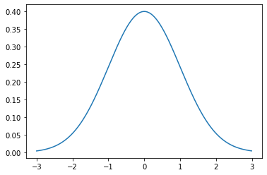
가우시안 그래프.

Multivariate Gaussian Distribution (다변량 정규 분포)

Multivariate Gaussian Distribution은 정규분포를 다차원 공간에 대해 확장한 분포이며, 식은 다음과 같습니다.

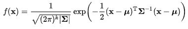
다변량 가우시안 식

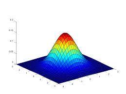
다변량 가우시안 그래프

Eigenvalue, Eigenvector, Covariance Matrix (고유값, 고유벡터, 공분산 행렬)

선형 대수에서 주로 사용하는 개념인 Eigenvalue, Eigenvector는 다음과 같은 식이 성립 합니다.

임의의 $n \times n$ 행렬 $A$ 에 대하여, 영벡터가 아닌 벡터 $\vec{x}$ 가 존재 한다면, 숫자 $\lambda$ 는 행렬 $A$ 의 고윳값이라고 할 수 있습니다.

A\vec{x} = \lambda\vec{x}

이 때, $\vec{x}$ 는 고윳값 $\lambda$ 에 대응하는 고유 벡터입니다.

이는 행렬의 법칙에 의해 다음과 같이 나타 낼 수 있습니다.

(A - \lambda)\vec{x} = 0

det(A - \lambda I) = 0

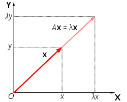
Eigenvalue, Eigenvector의 관계

여기서 Eigenvalue는 **"얼마 만큼 크기가 변했냐"**를 의미합니다. 그리고 Eigenvector는 행렬을 사영했을 때 **"원래 벡터와 평행한 벡터는 무엇인지"**를 의미 합니다. 그렇기 때문에, 각 특징 간의 공분산 (feature와 feature 사이의 연관성)을 나타내는 Covariance Matrix에 대해 높은 Eigenvalue를 가진 Eigenvector은 주성분 분석(PCA) 를 통해 학습 시 차원을 줄이는 데 사용 됩니다.

여기서 말하는 Covariance Matrix에 대해 추가 설명을 덧붙이자면, 대각 성분은 feature의 분산을 나타내고, 나머지는 각 행과 열에 대응하는 Covariance (각 feature의 선형 종속성) 를 나타 냅니다.

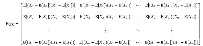
Covariance Matrix

Eigenvalue, Eigenvector

array = [[1, 2], [3, 4]]
eigenvalues, eigenvectors = np.linalg.eig(array)  # Eigenvalue, Eigenvector of Covarience Matrix

print("eigenvalue: ", eigenvalues)
print("eigenvector: ", eigenvectors)
print("eigenvalue * eigenvector: ", eigenvalues * eigenvectors)
print("array * eigenvector: ", array @ eigenvectors)

eigenvalue:  [-0.37228132  5.37228132]
eigenvector:  [[-0.82456484 -0.41597356]
 [ 0.56576746 -0.90937671]]
eigenvalue * eigenvector:  [[ 0.30697009 -2.23472698]
 [-0.21062466 -4.88542751]]
array * eigenvector:  [[ 0.30697009 -2.23472698]
 [-0.21062466 -4.88542751]]

Eigen Vector, Eigen Value, PCA

array = np.random.multivariate_normal([0, 0], [[1, 0], [0, 100]], 1000)  # multivariate (mean, covarience matrix, samples)
cov = np.cov(array.T)  # Covarience Matrix ((index x, index y) x에 대해, y가 얼마나 변화 하는가?)
print(cov)
eigenvalues, eigenvectors = np.linalg.eig(cov)  # Eigenvalue, Eigenvector of Covarience Matrix

print("eigenvalue: ", eigenvalues)
print("eigenvector: ", eigenvectors)

plt.scatter(array[:, 0], array[:, 1])
plt.quiver([0, 0], [0, 0], eigenvectors[:, 0], eigenvectors[:, 1], color=['r', 'b'], scale=3)
plt.xlim(-50, 50)
plt.ylim(-50, 50)
plt.show()

[[ 1.02530381  0.23267569]
 [ 0.23267569 97.82469968]]
eigenvalue:  [ 1.02474454 97.82525895]
eigenvector:  [[-0.99999711 -0.00240367]
 [ 0.00240367 -0.99999711]]

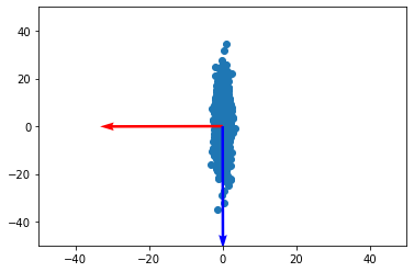
주성분은 파란색 벡터에 가까운걸, 수치적으로, 시각적으로 알 수 있다.

Differentiation in computer

Machine Learning에서 미분은 어떤 것을 의미 할까요? 이는 Cost Function에 대한 **Gradient descent (경사 하강법)**을 사용 할 때 사용합니다. 이는 컴퓨터에서 미분은 수식을 사용하는 해석적 방법이 아닌, 직접 값을 계산하여 진행하는 수치적 미분을 진행 합니다. 이를 구현하면 다음과 같습니다.

def diff(f, index, *args):  # index 번째의 parameter에 대해 편미분
    delta = 1e-4  # h
    new_args = list(args)  # index 번째의 parameter에 대해 delta를 더해 줌
    new_args[index] += delta
    return (f(*new_args) - f(*args)) / delta  # f(x + h, y) - f(x, y) / h

diff(lambda x, y: x ** 2 + y ** 2, 0, 3, 3)  # f(x, y) = x^2 + y^2

6.000099999994291

이를 그래프로 확인 해 보면 다음과 같습니다.

# 원래 그래프
x = np.arange(-3,3,.01)
y = x ** 2

# tangent, 접선
d = diff(lambda x: x ** 2, 0, 1)
x_tangent = np.arange(0, 2, .01)
y_tangent = (x_tangent - 1) * d + 1

# 그래프 표현
plt.plot(x, y)
plt.plot(x_tangent, y_tangent, color='r')
plt.show()

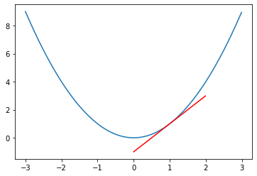
그래프로 표현 된 모습.

Computational Graph

Cost Function에 대한 **Gradient descent (경사 하강법)**을 사용 할 때, 매개변수에 상대적인 미분 값을 전달하기 위하기 위해선 어떤 것이 필요 할까요? 이럴 때는 계산 그래프를 사용합니다.

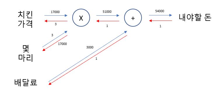
특정 매개변수가 변화 했을 때, 결과 값이 얼마만큼 움직이는 가?

곱셈 노드의 구현, 덧셈 노드의 구현 및 순전파는 다음과 같습니다.

class MulLayer:  # 곱셈 노드
    def forward(self, x, y):
        self.x = x
        self.y = y
        out = x * y
        
        return out
    
    def backward(self, dout):
        dx = dout * self.y
        dy = dout * self.x
        
        return dx, dy


class AddLayer:  # 덧셈 노드
    def forward(self, x, y):
        out = x + y
        return out
    
    def backward(self, dout):
        dx = dout * 1
        dy = dout * 1
        return dx, dy

chicken = 17000
num = 3
delivary_fee = 3000

mul_chicken = MulLayer()
add_fee = AddLayer()

chicken_price = mul_chicken.forward(chicken, num)
total_price = add_fee.forward(chicken_price, delivary_fee)
print(total_price)

역전파는 다음과 같습니다.

d_price = 1
d_chicken_price, d_delivary_fee = add_fee.backward(d_price)
d_chicken, d_num = mul_chicken.backward(d_chicken_price)

print("d_chicken_price: ", d_chicken_price)
print("d_delivary_fee: ", d_delivary_fee)
print("d_chicken: ", d_chicken)
print("d_num: ", d_num)

d_chicken_price:  1
d_delivary_fee:  1
d_chicken:  3
d_num:  17000

마치며

오늘은 이렇게 딥러닝에서 사용 되는 수학 공식들을 numpy를 이용 하여 구해 보았습니다. 다음 시간에는 Pandas의 사용 법에 대해 알아보도록 하겠습니다.