Archive된 사유는 다음 중 하나에 해당 됩니다.
- 작성 된지 너무 오랜 시간이 경과 하여, API가 변경 되었을 가능성이 높은 경우
- 주인장의 Data Engineering으로의 변경으로 질문의 답변이 어려워진 경우
- 글의 퀄리티가 좋지 않아 글을 다시 작성 할 필요가 있을 경우
Pandas
안녕하세요? Justkode 입니다. 오늘은 Pandas에 대해서 심층있게 알아보는 시간을 가져보도록 하겠습니다.
Pandas는 데이터 분석을 위해 만들어진 라이브러리로 Numpy와 함께 많이 사용 됩니다. 주로 사용하는 데이터 구조는 Dataframe과 Series로, Table 정보와 같은 데이터를 처리 하는데 이점이 있습니다.
Series and DataFrame
첫 번째로 Series입니다. Series는 1차원 배열의 형태를 가지며, Index라는 기준에 의해 데이터가 저장 된다고 보면 됩니다.
두 번째로 DataFrame입니다. DataFrame은 2차원 배열의 형태를 가지며, Index 와 Column 이라는 기준에 의해 데이터가 저장됩니다. 여기서 Column 으로 Indexing을 한 값은 Series입니다. 즉, DataFrame은 **"동일한 Index를 가진 Series의 조합"**이라고 봐도 무방합니다.
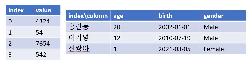
왼쪽은 Series를 나타내고, 오른쪽은 DataFrame을 나타낸다.
Series Code Implementation
Series 객체를 생성 할때는, pd.Series()를 이용 합니다. 파라미터로는 list, 1차원의 np.ndarray 객체가 들어 갈 수 있습니다. 아래 코드의 s_with_index 처럼, Series에 Index를 삽입 해 줄 수 있습니다.
In
import numpy as np
import pandas as pd

# Series 생성
s = pd.Series([1, 3, 5, 7, 9, 11])
s_with_index = pd.Series([1, 3, 5, 7, 9, 11], index=list("abcdef"))  # index를 임의로 삽입 해 줄 수 있다.

print(s)
print(s_with_index)
Out
0     1
1     3
2     5
3     7
4     9
5    11
dtype: int64
a     1
b     3
c     5
d     7
e     9
f    11
dtype: int64
DataFrame Code Implementation
DataFrame 객체를 생성 할때는, pd.DataFrame()을 이용 합니다. 파라미터로는 dict 객체가 들어 갈 수 있습니다. 아래 코드의 처럼, DataFrame에 Index를 삽입 해 줄 수 있습니다. 또한, 날짜 데이터 (혹은 배열)을 삽입 할때에는 pd.to_datetime() 함수를 이용하여, str 객체 로부터, datetime 객체로의 형변환이 가능합니다.
In
# DataFrame 생성
df = pd.DataFrame({
    "age": [20, 12, 1],
    "birth": pd.to_datetime(["2002-01-01", "2010-07-19", "2021-03-05"]),  # datetime 형변환
    "gender": ["Male", "Male", "Female"]
}, index=["홍길동", "이기영", "신짱아"])
df
Out
| age | birth | gender | |
|---|---|---|---|
| 홍길동 | 20 | 2002-01-01 | Male |
| 이기영 | 12 | 2010-07-19 | Male |
| 신짱아 | 1 | 2021-03-05 | Female |
Series의 집합은 DataFrame
다음과 같이 DataFrame 객체에 대한 Column Indexing을 통해, Series를 추출 할 수 있습니다.
In
print(type(df['birth']))
df['birth']  # DataFrame은 Series의 집합
Out
<class 'pandas.core.series.Series'>

홍길동   2002-01-01
이기영   2010-07-19
신짱아   2021-03-05
Name: birth, dtype: datetime64[ns]
Datetime Index
다음과 같이 Datetime으로 이루어진 Index 객체를 만들 수 있습니다.
In
dates = pd.date_range("20130101", periods=6)  # Datatimes Index
print(type(dates))
dates
Out
<class 'pandas.core.indexes.datetimes.DatetimeIndex'>

DatetimeIndex(['2013-01-01', '2013-01-02', '2013-01-03', '2013-01-04',
                '2013-01-05', '2013-01-06'],
                dtype='datetime64[ns]', freq='D')
Read CSV, Head, Tail
pd.read_csv()를 이용하여, csv 파일을 읽어, DataFrame 형식으로 만들 수 있습니다. 또한, DataFrame.head() 혹은 DataFrame.tail()을 통해, 상위 n개 (파라미터를 삽입하지 않을 시 5개) 혹은, 하위 n개 (파라미터를 삽입하지 않을 시 5개)를 열람 할 수 있습니다.
In
df2 = pd.read_csv('./iris.csv')
df2.head(3)  # 상위 3개, default 5개
Out
| sepal.length | sepal.width | petal.length | petal.width | variety | |
|---|---|---|---|---|---|
| 0 | 5.1 | 3.5 | 1.4 | 0.2 | Setosa |
| 1 | 4.9 | 3.0 | 1.4 | 0.2 | Setosa |
| 2 | 4.7 | 3.2 | 1.3 | 0.2 | Setosa |
In
df2.tail(4) # 하위 4개, default 5개Out
| sepal.length | sepal.width | petal.length | petal.width | variety | |
|---|---|---|---|---|---|
| 146 | 6.3 | 2.5 | 5.0 | 1.9 | Virginica |
| 147 | 6.5 | 3.0 | 5.2 | 2.0 | Virginica |
| 148 | 6.2 | 3.4 | 5.4 | 2.3 | Virginica |
| 149 | 5.9 | 3.0 | 5.1 | 1.8 | Virginica |
Transposition
다음과 같이 행과 열이 뒤바뀐 전치 DataFrame을 열람 할 수 있습니다.
In
df2.T # 행, 열 전치Out
| 0 | 1 | 2 | 3 | 4 | 5 | 6 | 7 | 8 | 9 | ... | 140 | 141 | 142 | 143 | 144 | 145 | 146 | 147 | 148 | 149 | |
|---|---|---|---|---|---|---|---|---|---|---|---|---|---|---|---|---|---|---|---|---|---|
| sepal.length | 5.1 | 4.9 | 4.7 | 4.6 | 5 | 5.4 | 4.6 | 5 | 4.4 | 4.9 | ... | 6.7 | 6.9 | 5.8 | 6.8 | 6.7 | 6.7 | 6.3 | 6.5 | 6.2 | 5.9 |
| sepal.width | 3.5 | 3 | 3.2 | 3.1 | 3.6 | 3.9 | 3.4 | 3.4 | 2.9 | 3.1 | ... | 3.1 | 3.1 | 2.7 | 3.2 | 3.3 | 3 | 2.5 | 3 | 3.4 | 3 |
| petal.length | 1.4 | 1.4 | 1.3 | 1.5 | 1.4 | 1.7 | 1.4 | 1.5 | 1.4 | 1.5 | ... | 5.6 | 5.1 | 5.1 | 5.9 | 5.7 | 5.2 | 5 | 5.2 | 5.4 | 5.1 |
| petal.width | 0.2 | 0.2 | 0.2 | 0.2 | 0.2 | 0.4 | 0.3 | 0.2 | 0.2 | 0.1 | ... | 2.4 | 2.3 | 1.9 | 2.3 | 2.5 | 2.3 | 1.9 | 2 | 2.3 | 1.8 |
| variety | Setosa | Setosa | Setosa | Setosa | Setosa | Setosa | Setosa | Setosa | Setosa | Setosa | ... | Virginica | Virginica | Virginica | Virginica | Virginica | Virginica | Virginica | Virginica | Virginica | Virginica |
5 rows × 150 columns
Describe
DataFrame.describe()를 통해서, DataFrame의 각 Column에 대한 대략적인 정보를 열람 할 수 있습니다.
In
df2.describe()Out
| sepal.length | sepal.width | petal.length | petal.width | |
|---|---|---|---|---|
| count | 150.000000 | 150.000000 | 150.000000 | 150.000000 |
| mean | 5.843333 | 3.057333 | 3.758000 | 1.199333 |
| std | 0.828066 | 0.435866 | 1.765298 | 0.762238 |
| min | 4.300000 | 2.000000 | 1.000000 | 0.100000 |
| 25% | 5.100000 | 2.800000 | 1.600000 | 0.300000 |
| 50% | 5.800000 | 3.000000 | 4.350000 | 1.300000 |
| 75% | 6.400000 | 3.300000 | 5.100000 | 1.800000 |
| max | 7.900000 | 4.400000 | 6.900000 | 2.500000 |
Sort Index
DataFrame.sort_index()를 이용하여, Index 기준으로 정렬 할 수 있습니다. axis에는 어떤 축을 중심으로 정렬 할 지, ascending은 오름차순 정렬 여부를 결정 하는데 사용 합니다.
In
df2.sort_index(axis=0, ascending=False)Out
| sepal.length | sepal.width | petal.length | petal.width | variety | |
|---|---|---|---|---|---|
| 149 | 5.9 | 3.0 | 5.1 | 1.8 | Virginica |
| 148 | 6.2 | 3.4 | 5.4 | 2.3 | Virginica |
| 147 | 6.5 | 3.0 | 5.2 | 2.0 | Virginica |
| 146 | 6.3 | 2.5 | 5.0 | 1.9 | Virginica |
| 145 | 6.7 | 3.0 | 5.2 | 2.3 | Virginica |
| ... | ... | ... | ... | ... | ... |
| 4 | 5.0 | 3.6 | 1.4 | 0.2 | Setosa |
| 3 | 4.6 | 3.1 | 1.5 | 0.2 | Setosa |
| 2 | 4.7 | 3.2 | 1.3 | 0.2 | Setosa |
| 1 | 4.9 | 3.0 | 1.4 | 0.2 | Setosa |
| 0 | 5.1 | 3.5 | 1.4 | 0.2 | Setosa |
150 rows × 5 columns
In
df2.sort_index(axis=1, ascending=False)Out
| variety | sepal.width | sepal.length | petal.width | petal.length | |
|---|---|---|---|---|---|
| 0 | Setosa | 3.5 | 5.1 | 0.2 | 1.4 |
| 1 | Setosa | 3.0 | 4.9 | 0.2 | 1.4 |
| 2 | Setosa | 3.2 | 4.7 | 0.2 | 1.3 |
| 3 | Setosa | 3.1 | 4.6 | 0.2 | 1.5 |
| 4 | Setosa | 3.6 | 5.0 | 0.2 | 1.4 |
| ... | ... | ... | ... | ... | ... |
| 145 | Virginica | 3.0 | 6.7 | 2.3 | 5.2 |
| 146 | Virginica | 2.5 | 6.3 | 1.9 | 5.0 |
| 147 | Virginica | 3.0 | 6.5 | 2.0 | 5.2 |
| 148 | Virginica | 3.4 | 6.2 | 2.3 | 5.4 |
| 149 | Virginica | 3.0 | 5.9 | 1.8 | 5.1 |
150 rows × 5 columns
Sort By Values
DataFrame.sort_values()를 이용하여, Value 기준으로 정렬 할 수 있습니다. by를 통해, 어떤 Column을 기준으로 정렬 할 지, ascending을 통해, 오름차순 정렬 여부를 고를 수 있습니다.
In
df2.sort_values(by="sepal.width")Out
| sepal.length | sepal.width | petal.length | petal.width | variety | |
|---|---|---|---|---|---|
| 60 | 5.0 | 2.0 | 3.5 | 1.0 | Versicolor |
| 62 | 6.0 | 2.2 | 4.0 | 1.0 | Versicolor |
| 119 | 6.0 | 2.2 | 5.0 | 1.5 | Virginica |
| 68 | 6.2 | 2.2 | 4.5 | 1.5 | Versicolor |
| 41 | 4.5 | 2.3 | 1.3 | 0.3 | Setosa |
| ... | ... | ... | ... | ... | ... |
| 16 | 5.4 | 3.9 | 1.3 | 0.4 | Setosa |
| 14 | 5.8 | 4.0 | 1.2 | 0.2 | Setosa |
| 32 | 5.2 | 4.1 | 1.5 | 0.1 | Setosa |
| 33 | 5.5 | 4.2 | 1.4 | 0.2 | Setosa |
| 15 | 5.7 | 4.4 | 1.5 | 0.4 | Setosa |
150 rows × 5 columns
Selection
DataFrame을 Index Slicing을 통해, Index 기준으로 데이터를 잘라 낼 수 있습니다.
In
df2[100:105] # index 기준으로 짜름Out
| sepal.length | sepal.width | petal.length | petal.width | variety | |
|---|---|---|---|---|---|
| 100 | 6.3 | 3.3 | 6.0 | 2.5 | Virginica |
| 101 | 5.8 | 2.7 | 5.1 | 1.9 | Virginica |
| 102 | 7.1 | 3.0 | 5.9 | 2.1 | Virginica |
| 103 | 6.3 | 2.9 | 5.6 | 1.8 | Virginica |
| 104 | 6.5 | 3.0 | 5.8 | 2.2 | Virginica |
loc
DataFrame.loc 에 대한 Indexing을 통해, 특정 행과 열에 대한 데이터를 추출 할 수 있습니다. 첫 번째 slicing은 행에 대한 slicing이고, 두 번째 slicing은 열에 대한 slicing입니다.
In
df2.loc[:, "sepal.length":"petal.length"]Out
| sepal.length | sepal.width | petal.length | |
|---|---|---|---|
| 0 | 5.1 | 3.5 | 1.4 |
| 1 | 4.9 | 3.0 | 1.4 |
| 2 | 4.7 | 3.2 | 1.3 |
| 3 | 4.6 | 3.1 | 1.5 |
| 4 | 5.0 | 3.6 | 1.4 |
| ... | ... | ... | ... |
| 145 | 6.7 | 3.0 | 5.2 |
| 146 | 6.3 | 2.5 | 5.0 |
| 147 | 6.5 | 3.0 | 5.2 |
| 148 | 6.2 | 3.4 | 5.4 |
| 149 | 5.9 | 3.0 | 5.1 |
150 rows × 3 columns
다음과 같이, Slicing 이 아닌, 특정 행 또는 열 요소에 일치하는 list 객체를 넣음으로써 해당하는 행 또는 열을 추출할 수 있습니다.
In
df2.loc[:, ["sepal.length", "petal.length"]]Out
| sepal.length | petal.length | |
|---|---|---|
| 0 | 5.1 | 1.4 |
| 1 | 4.9 | 1.4 |
| 2 | 4.7 | 1.3 |
| 3 | 4.6 | 1.5 |
| 4 | 5.0 | 1.4 |
| ... | ... | ... |
| 145 | 6.7 | 5.2 |
| 146 | 6.3 | 5.0 |
| 147 | 6.5 | 5.2 |
| 148 | 6.2 | 5.4 |
| 149 | 5.9 | 5.1 |
150 rows × 2 columns
In
df2.loc[[0, 100], ["sepal.length", "petal.length"]]Out
| sepal.length | petal.length | |
|---|---|---|
| 0 | 5.1 | 1.4 |
| 100 | 6.3 | 6.0 |
list 객체가 아닌, 해당하는 요소만 넣어서 추출 또한 가능 합니다.
In
df2.loc[0, ["sepal.length", "petal.length"]]Out
sepal.length    5.1
petal.length    1.4
Name: 0, dtype: object
In
df2.loc[0, "sepal.length"]Out
5.1At
DataFrame.at을 이용하여, 행과 열을 입력하여 특정 Scala 값에 빠르게 접근 할 수 있습니다.
In
df2.at[0, "sepal.length"] # fast accessOut
5.1iloc
DataFrame.iloc을 이용하여, 숫자를 통해 행 또는 열에 접근 할 수 있습니다.
In
df2.iloc[3:5, 0:2]Out
| sepal.length | sepal.width | |
|---|---|---|
| 3 | 4.6 | 3.1 |
| 4 | 5.0 | 3.6 |
Boolean Indexing
특정 조건을 만족하는 행을 추출 하고 싶을 때는 어떻게 하면 될까요? 그럴 때 사용 하는 것이 Boolean Indexing 입니다. 원리는 다음과 같습니다.
- Series 객체에 조건문을 적용 시, 조건에 해당 하는 index에는 True가, 그렇지 않은 index에는 False가 반환 된다.
- 만약 이를 DataFrame 객체에 대해 Indexing을 시도하면, True를 반환한 Index에 대해서만 추출을 하게 된다. 이를 Boolean Indexing 이라고 한다.
- 따라서, 아래와 같이 코드를 작성시, 조건문을 만족하는 Row들만 남게 된다.
In
df2[df2["sepal.length"] > 5] # if sepal.length, boolean indexingOut
| sepal.length | sepal.width | petal.length | petal.width | variety | |
|---|---|---|---|---|---|
| 0 | 5.1 | 3.5 | 1.4 | 0.2 | Setosa |
| 5 | 5.4 | 3.9 | 1.7 | 0.4 | Setosa |
| 10 | 5.4 | 3.7 | 1.5 | 0.2 | Setosa |
| 14 | 5.8 | 4.0 | 1.2 | 0.2 | Setosa |
| 15 | 5.7 | 4.4 | 1.5 | 0.4 | Setosa |
| ... | ... | ... | ... | ... | ... |
| 145 | 6.7 | 3.0 | 5.2 | 2.3 | Virginica |
| 146 | 6.3 | 2.5 | 5.0 | 1.9 | Virginica |
| 147 | 6.5 | 3.0 | 5.2 | 2.0 | Virginica |
| 148 | 6.2 | 3.4 | 5.4 | 2.3 | Virginica |
| 149 | 5.9 | 3.0 | 5.1 | 1.8 | Virginica |
118 rows × 5 columns
Is in?
DataFrame.isin() 혹은 Series.isin()은, 파라미터로 들어간 iterate 객체에 대해, 해당 하는 값을 가지고 있는 경우, True를 반환하고, 그렇지 않은 값에 대해서는 False를 반환하는 함수 입니다. 위에서 언급한 Boolean Indexing을 하는데 사용 됩니다.
In
df2[df2["sepal.length"].isin([5.0, 5.3])]Out
| sepal.length | sepal.width | petal.length | petal.width | variety | |
|---|---|---|---|---|---|
| 4 | 5.0 | 3.6 | 1.4 | 0.2 | Setosa |
| 7 | 5.0 | 3.4 | 1.5 | 0.2 | Setosa |
| 25 | 5.0 | 3.0 | 1.6 | 0.2 | Setosa |
| 26 | 5.0 | 3.4 | 1.6 | 0.4 | Setosa |
| 35 | 5.0 | 3.2 | 1.2 | 0.2 | Setosa |
| 40 | 5.0 | 3.5 | 1.3 | 0.3 | Setosa |
| 43 | 5.0 | 3.5 | 1.6 | 0.6 | Setosa |
| 48 | 5.3 | 3.7 | 1.5 | 0.2 | Setosa |
| 49 | 5.0 | 3.3 | 1.4 | 0.2 | Setosa |
| 60 | 5.0 | 2.0 | 3.5 | 1.0 | Versicolor |
| 93 | 5.0 | 2.3 | 3.3 | 1.0 | Versicolor |
Data Assign
at, iat, loc, iloc 을 이용해 추출한 행, 열, 혹은 스칼라 값에 대해 특정 값을 대입 할 수 있습니다.
In
df2.at[0, "sepal.length"] = 5
df2.iat[0, 1] = 4
df2.loc[:, "sepal.length"] = 5
df2
Out
| sepal.length | sepal.width | petal.length | petal.width | variety | |
|---|---|---|---|---|---|
| 0 | 5 | 4.0 | 1.4 | 0.2 | Setosa |
| 1 | 5 | 3.0 | 1.4 | 0.2 | Setosa |
| 2 | 5 | 3.2 | 1.3 | 0.2 | Setosa |
| 3 | 5 | 3.1 | 1.5 | 0.2 | Setosa |
| 4 | 5 | 3.6 | 1.4 | 0.2 | Setosa |
| ... | ... | ... | ... | ... | ... |
| 145 | 5 | 3.0 | 5.2 | 2.3 | Virginica |
| 146 | 5 | 2.5 | 5.0 | 1.9 | Virginica |
| 147 | 5 | 3.0 | 5.2 | 2.0 | Virginica |
| 148 | 5 | 3.4 | 5.4 | 2.3 | Virginica |
| 149 | 5 | 3.0 | 5.1 | 1.8 | Virginica |
150 rows × 5 columns
In
df2.loc[df2["sepal.width"] > 3, "sepal.length"] = 3  # Number of True
df2
Out
| sepal.length | sepal.width | petal.length | petal.width | variety | |
|---|---|---|---|---|---|
| 0 | 3 | 4.0 | 1.4 | 0.2 | Setosa |
| 1 | 5 | 3.0 | 1.4 | 0.2 | Setosa |
| 2 | 3 | 3.2 | 1.3 | 0.2 | Setosa |
| 3 | 3 | 3.1 | 1.5 | 0.2 | Setosa |
| 4 | 3 | 3.6 | 1.4 | 0.2 | Setosa |
| ... | ... | ... | ... | ... | ... |
| 145 | 5 | 3.0 | 5.2 | 2.3 | Virginica |
| 146 | 5 | 2.5 | 5.0 | 1.9 | Virginica |
| 147 | 5 | 3.0 | 5.2 | 2.0 | Virginica |
| 148 | 3 | 3.4 | 5.4 | 2.3 | Virginica |
| 149 | 5 | 3.0 | 5.1 | 1.8 | Virginica |
150 rows × 5 columns
Operations
DataFrame의 mean(), max(), min() 등의 함수를 이용하여, 대략적인 행 또는 열에 대한 통계 자료를 볼 수 있습니다.
In
df2.mean()Out
sepal.length    4.106667
sepal.width     3.060667
petal.length    3.758000
petal.width     1.199333
dtype: float64
In
df2.mean(1) # Row에 대한 통계Out
0      2.150
1      2.400
2      1.925
3      1.950
4      2.050
        ...
145    3.875
146    3.600
147    3.800
148    3.525
149    3.725
Length: 150, dtype: float64
Apply
DataFrame.apply()를 통해, 파라미터에 함수 객체를 넣음으로써, DataFrame의 Element 전체에 함수를 적용 할 수 있습니다.
In
df2.apply(lambda x: (x - x.min())/(x.max() - x.min()) if x.name in ['sepal.width', 'petal.length'] else x)Out
| sepal.length | sepal.width | petal.length | petal.width | variety | |
|---|---|---|---|---|---|
| 0 | 3 | 0.833333 | 0.067797 | 0.2 | Setosa |
| 1 | 5 | 0.416667 | 0.067797 | 0.2 | Setosa |
| 2 | 3 | 0.500000 | 0.050847 | 0.2 | Setosa |
| 3 | 3 | 0.458333 | 0.084746 | 0.2 | Setosa |
| 4 | 3 | 0.666667 | 0.067797 | 0.2 | Setosa |
| ... | ... | ... | ... | ... | ... |
| 145 | 5 | 0.416667 | 0.711864 | 2.3 | Virginica |
| 146 | 5 | 0.208333 | 0.677966 | 1.9 | Virginica |
| 147 | 5 | 0.416667 | 0.711864 | 2.0 | Virginica |
| 148 | 3 | 0.583333 | 0.745763 | 2.3 | Virginica |
| 149 | 5 | 0.416667 | 0.694915 | 1.8 | Virginica |
150 rows × 5 columns
Histograming
특정 범위에 몇개의 데이터가 있는지 판단하기 위해선 뭐가 필요 할까요? 이럴 때는 pd.cut을 이용합니다. 첫 번째 파라미터로는 Series혹은 DataFrame을 받고, 두 번째 파라미터로는 범위를 가진 list를 입력 받습니다. 그 다음 이에 대해 pd.value_counts()에 pd.cut으로 만든 객체를 넣어 Series 객체를 확인 할 수 있습니다.
In
factor = pd.cut(df2['petal.width'], [0, 1, 2, 3])
pd.value_counts(factor)
Out
(1, 2]    70
(0, 1]    57
(2, 3]    23
Name: petal.width, dtype: int64
Concat
pd.concat을 통해서, 같은 Column 을 가진 DataFrame을 연결 할 수 있습니다.
In
pd.concat([df2[:5], df2[10:15], df2[20:25]])Out
| sepal.length | sepal.width | petal.length | petal.width | variety | |
|---|---|---|---|---|---|
| 0 | 3 | 4.0 | 1.4 | 0.2 | Setosa |
| 1 | 5 | 3.0 | 1.4 | 0.2 | Setosa |
| 2 | 3 | 3.2 | 1.3 | 0.2 | Setosa |
| 3 | 3 | 3.1 | 1.5 | 0.2 | Setosa |
| 4 | 3 | 3.6 | 1.4 | 0.2 | Setosa |
| 10 | 3 | 3.7 | 1.5 | 0.2 | Setosa |
| 11 | 3 | 3.4 | 1.6 | 0.2 | Setosa |
| 12 | 5 | 3.0 | 1.4 | 0.1 | Setosa |
| 13 | 5 | 3.0 | 1.1 | 0.1 | Setosa |
| 14 | 3 | 4.0 | 1.2 | 0.2 | Setosa |
| 20 | 3 | 3.4 | 1.7 | 0.2 | Setosa |
| 21 | 3 | 3.7 | 1.5 | 0.4 | Setosa |
| 22 | 3 | 3.6 | 1.0 | 0.2 | Setosa |
| 23 | 3 | 3.3 | 1.7 | 0.5 | Setosa |
| 24 | 3 | 3.4 | 1.9 | 0.2 | Setosa |
Merge
pd.merge를 통해서, 두 개의 DataFrame에 대해 같은 키 값을 가진 행을 연결 해 줄 수 있습니다.
In
left = pd.DataFrame({"key": ["foo", "bar"], "lval": [1, 2]})
right = pd.DataFrame({"key": ["foo", "bar"], "rval": [4, 5]})

pd.merge(left, right, on="key")
Out
| key | lval | rval | |
|---|---|---|---|
| 0 | foo | 1 | 4 |
| 1 | bar | 2 | 5 |
Group By
DataFrame.groupby를 통해, 특정 열에 대해 같은 값을 가진 행끼리 묶어서 Groupby 객체를 만들 수 있습니다. 이러한 Groupby 된 객체로, 평균, 최대, 최소, 분산 등의 값을 추출 할 수 있습니다.
In
df2.groupby(['variety']).mean()Out
| sepal.length | sepal.width | petal.length | petal.width | |
|---|---|---|---|---|
| variety | ||||
| Setosa | 3.32 | 3.438 | 1.462 | 0.246 |
| Versicolor | 4.68 | 2.770 | 4.260 | 1.326 |
| Virginica | 4.32 | 2.974 | 5.552 | 2.026 |
두 개 이상의 열에 대해서도 Groupby가 가능합니다.
In
df = pd.DataFrame(
     {
         "A": ["foo", "bar", "foo", "bar", "foo", "bar", "foo", "foo"],
         "B": ["one", "one", "two", "three", "two", "two", "one", "three"],
         "C": np.random.randn(8),
         "D": np.random.randn(8),
     }
)

df.groupby(["A", "B"]).sum()
Out
| C | D | ||
|---|---|---|---|
| A | B | ||
| bar | one | -0.377903 | -0.623514 |
| three | -0.391103 | 0.620304 | |
| two | 0.920777 | -0.561905 | |
| foo | one | 1.647783 | -1.258050 |
| three | -0.329915 | 0.798162 | |
| two | -2.269855 | -1.696683 |
Plotting
matplotlib.pyplot에 대한 특별한 함수 작성 없이, DataFrame내부의 plot()을 이용하여, 간편하게 시각화 하여 볼 수 있습니다.
In
import matplotlib.pyplot as plt

df3 = pd.DataFrame({
    'A': np.random.randn(4),
    'B': np.random.randn(4)
}, index=list('abcd'))
df3.plot()
Out
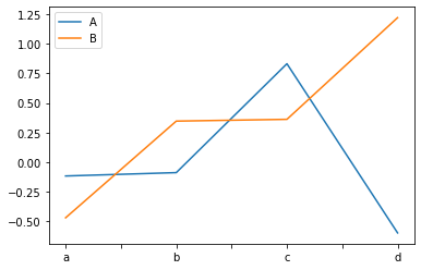
DataFrame을 촐력 한 모습
Histogram 또한 볼 수 있습니다.
df = pd.DataFrame(
    np.random.randint(1, 7, 6000),
    columns = ['one'])
df['two'] = df['one'] + np.random.randint(1, 7, 6000)
ax = df.plot.hist(bins=12, alpha=0.5)
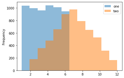
DataFrame에 대한 histogram을 출력 한 모습
마치며
이 게시글은 10 Minutes to Pandas를 참고 하여 만들어 졌습니다. 여기에 있는 내용들은 모두 기초 사용법을 흐름에 따라 간 것일 뿐입니다. 더 많은 API, 더 많은 정보들은 필요 할 때마다 구글에서 개인적으로 많이 찾아보는 것을 권장합니다. 다음 시간에는 matplotlib에 대해서 공부 해 보겠습니다. 감사합니다.